


Bitcoin has never ended a year on a positive note after such a bad start.
Bitcoin seasonality is one of those market stories that lives on because it’s easy to screenshot average values. The problem is that averages often hide the only thing that matters: the state.
A strong “uptober” in a healthy bullish trend is not the same trade as a strong October after a year of spending the first quarter underwater. If the median for the month is still negative, there is no advantage in having a positive December average. And if the market has already pushed most of its upside, a hot first quarter is not automatically a continuation signal.
That’s the core result here. The calendar is not the only useful part of Bitcoin price seasonality. interaction between month, administrationand path is much more important.
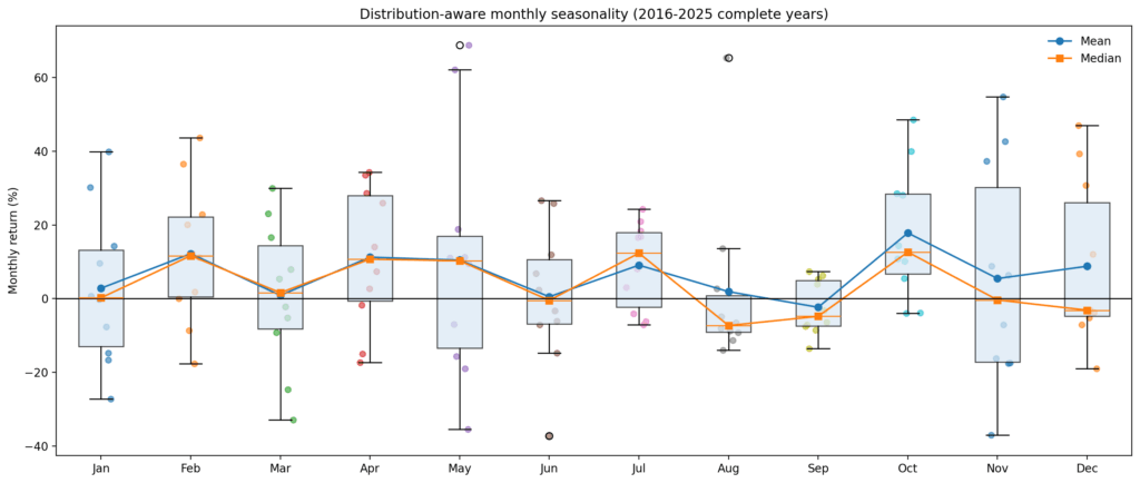
The first problem with talking about seasonality is that the mean flattens the distribution.
If we look only at average monthly returns, Bitcoin appears to offer a menu of repeating bullish windows. In the latest sample, October stands out with an average return of 17.8%, median 12.7%, and win rate of 80%. July continued to perform well, with an average return of 9.1%, a median return of 12.4%, and a win rate of 70%. February and April are also looking pretty positive.
But above average, things change quickly.
August is the most obvious example. The average return is slightly positive at 1.9%, which sounds good until you look underneath. The median is -7.3%, the win rate is only 30%, and the distribution is positively skewed.
To put it simply, August was not a reliable “good month.” This has been a low hit month, but it has been rescued from time to time by some big upticks.
In December, the same problem occurs in a softer form. The average value is positive, but the median value is negative, and the win rate is only 40%. The same goes for November. The headline is a positive average, but the distribution is well diversified and has a downward tail, so the average is much better than the actual experience of holding the risk over that period.
May is also a trap. Although the average return looks healthy, month-to-month variation dominates. The upward tail is large, the downward tail is large, and the standard deviation is high enough that just saying “May is positive on average” tells us little about what kind of risk you are actually taking.
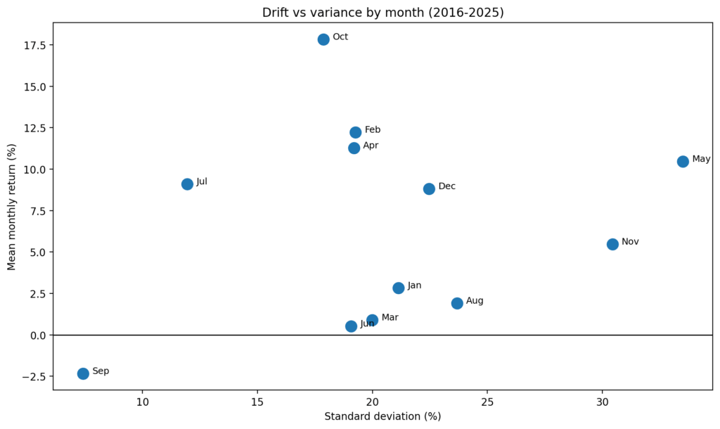
some months are Drift dominancethe mean, median, and win rate are almost in line. Others distributed dominanton average, is doing more storytelling than prediction.

The month that seems most useful is not the one most people talk about.
The prettiest month is October. Not because it always works (it doesn’t), but because the mean, median, and win rate all point in the same direction.
The next best example is July. These are the closest thing to a stable seasonal window in our data.
In contrast, some of the more familiar seasonal topics seem fragile.
The positive mean value in August is mostly due to skewness. November and December also work, but they are not trending months in a statistical sense. These are conditional months and require confirmation from the regime and path.
That’s the first big dividing line between edge and illusion. A month with a positive average is not necessarily a month with a reproducible edge.
If the median is negative and the win rate is low, there is no seasonality. What you have is optionality disguised as consistency.

The regime changes the sign of seasonal signals
The next step was to divide the year into objective regimes. That is, bullish years with annual returns above 50%, bearish years with annual returns below -20%, and neutral years in between.
Once you do this, unconditional seasonality begins to look more like a mixed average of opposite states than a structure.
Some months reverse sign depending on the regime, such as January, March, May, June, August, November, and December.
In other words, the same month that looks strong in the sample as a whole can turn negative when isolated against a weaker macro background.
This is exactly what would be expected if seasonality were downstream rather than independent of market conditions.
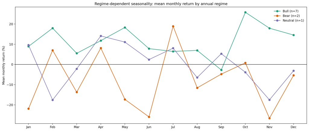
There are only a few months in which any administration looks relatively resilient. July is the best candidate. April is also somewhat constructive, but not very pretty. Meanwhile, September remains sufficiently weak across major regimes that it deserves to be respected as a recurrent patch of weakness rather than a one-time anomaly.
The caveat is obvious. This means that the number of bear samples is small. But that’s also the point. If a seasonality claim collapses the moment you ask whether it persists in different states of the world, then it probably wasn’t a strong claim to begin with.

The real strength is path dependence, not calendar myths
The strongest signal is not the monthly average. These are state variables associated with the passage of years.
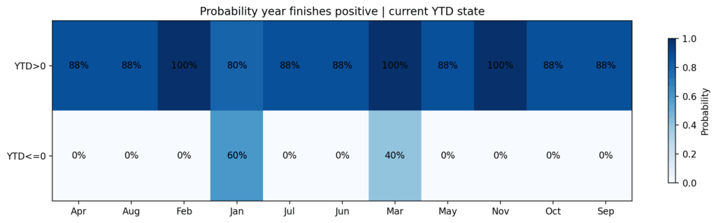
In the 2016-2025 sample, if Bitcoin was positive year-to-date after February, it ended the year positive 7 out of 7 times.
In the case of a year-to-date negative figure since February, it ended with a positive zero out of three times.
After March, this division remained acute. YTD-plus years ended positive 5 out of 5 times, while only 2 out of 5 YTD-negative years ended positive.
It’s not a trivial difference. This suggests that by late Q1, Bitcoin’s seasonal profile is already filtered by whether the year is on a healthy trend or in repair mode.
The market isn’t just having a “good” or “bad” month. Entering them from a certain state, the forward distribution changes.
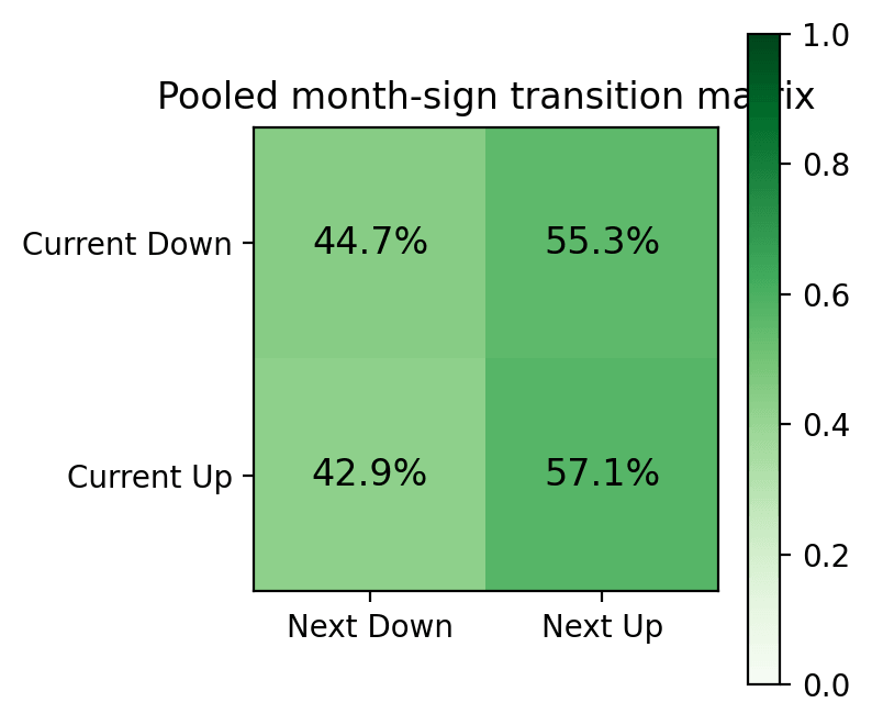
Just as importantly, simple monthly sign momentum cannot be sustained. After an up month, the next month was positive 57.1% of the time. After a weak month, the next month was positive 55.3% of the time. It’s not a serious edge.
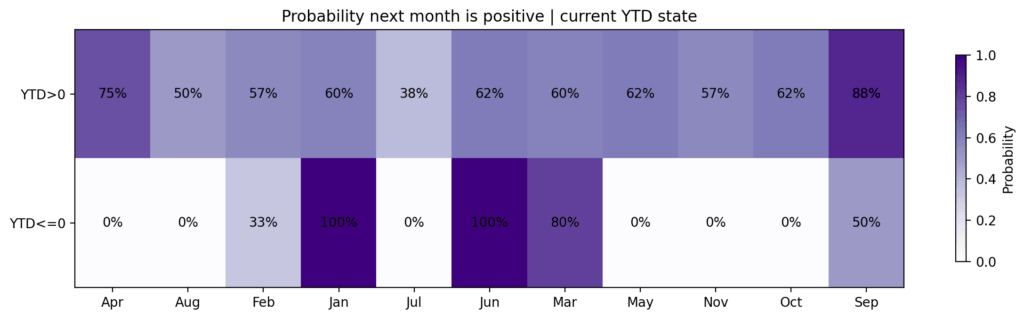
Useful signals will only emerge conditional on the broader path, year-to-date trajectory, first-quarter results, and whether the year is trending toward recovery or collapse.
A strong first quarter helps the year, but often hurts the next quarter.
One of the more interesting findings is that strong performance at the beginning of the year is not a clear signal of continuation.
Every year that saw a first-quarter return of more than 20% ended positive. However, the second quarter at the time was weaker, with an average decline of 15.1%.
This is important because it is the turning point. direction from timing.
The strong first quarter results increased the likelihood of positive full-year results, but also tended to increase the likelihood of future profit extraction and spring spending.
In other words, while the market remains structurally constructive, tactical ownership may become more difficult heading into the second quarter.
The data here does not support the jump that a positive trend at the annual level is a positive entry signal for the next month or quarter.
June seems like a real decision node.
If your data has a real seasonal checkpoint, it’s not just for a single month, but for the year through mid-year. No year with a first-half return below zero ended positive. Seven out of eight years ended with positive first-half earnings, with 2025 being the exception.
The same logic appears in a year with a negative first quarter. If the second quarter recovers by more than 20% after a weak first quarter, full-year results have improved significantly.
If rebounding didn’t meet that standard, you couldn’t finish the year with a positive score. It won’t decide the fate of the second quarter, but it will certainly be the most profitable repair period of the year.
Its meaning is simple and clear. Once a year, when an opened item is damaged, the burden of proof shifts to the second quarter.
If the market is not able to meaningfully repair itself by June, there is much less reason to rely on seasonal optimism for the second half of the year.
Why 2026 matters now
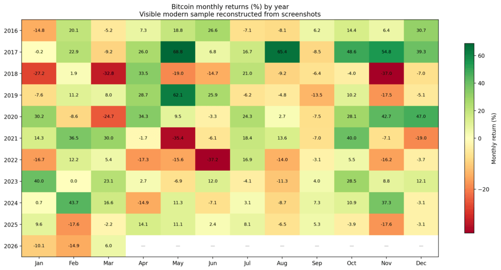
This framework is particularly relevant in 2026. Because this year, one of the cleaner modern pass templates has already been broken.
Every year, when January is negative, February is positive. This is until now.
2026 began with a 10% decline in January, a further 14.8% decline in February, and then a 6% recovery by mid-March, resulting in a decline of around 19% in the first quarter.
This negative-negative-positive order is unusual in modern samples, and 2026 is best described as a fix-or-break situation.
Cluster analysis maps the current year closest to a group that includes 2016, 2018, 2022, and 2025.
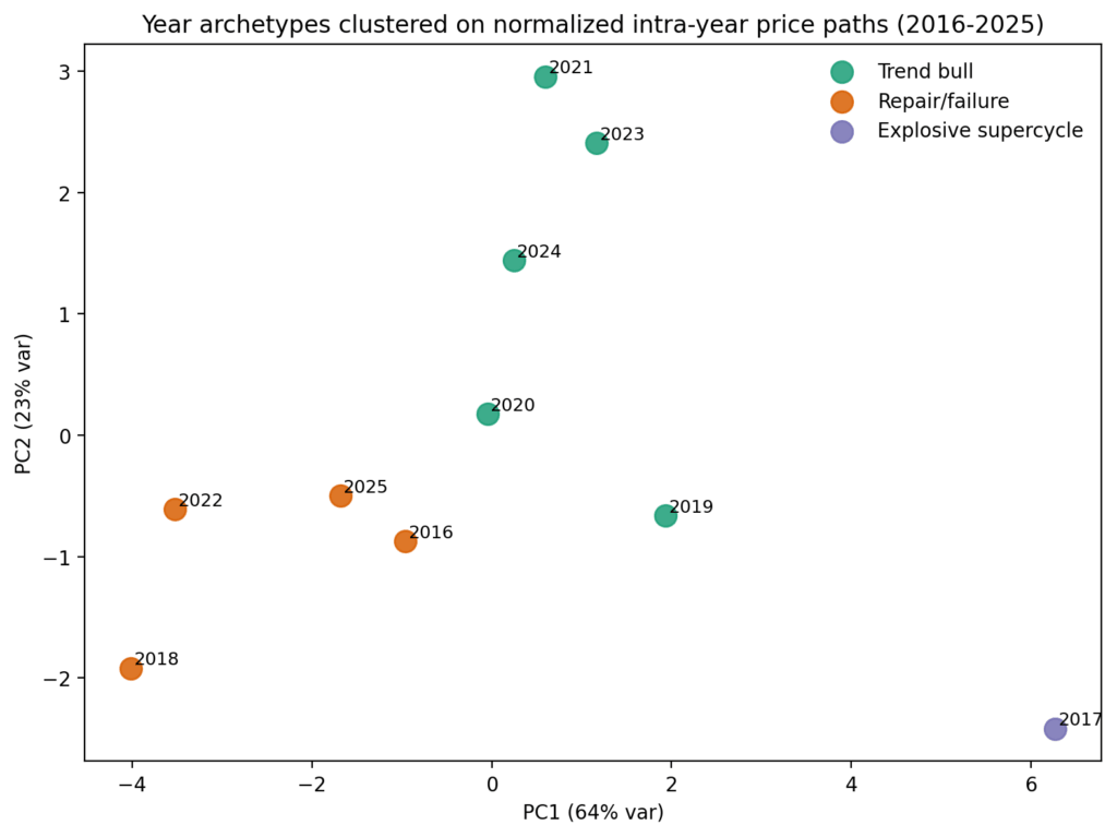
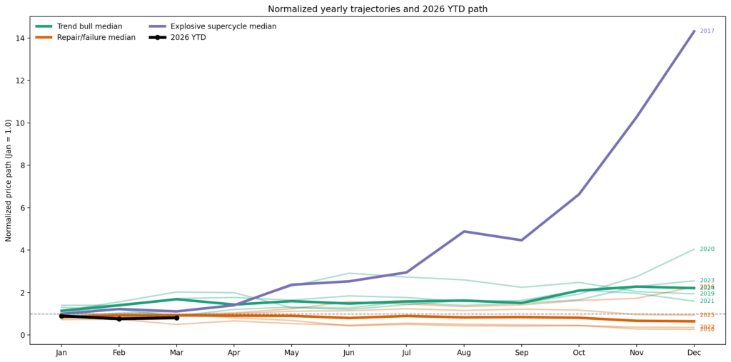
The correct frame for 2026 is one year of successful repair, two years of failure, and one year of rebound with no trend. It’s not “Bitcoin usually does well in Q4” or “March bounced so the worst is over” but rather “Will Q2 do enough to get us out of a damaged year?”
2026 scenario tree is a remediation test, not a seasonal layup
The most bullish direction from here is a full-scale repair system. It looks set for a strong recovery in the second quarter, a summer digest, and a pick-up again heading into the second half of the year.
Historically, the closest is 2016, and 2020 is an outlier for a more explosive rise.
Bitcoin would need to compound by more than 20% in the second quarter to return to more than flat from current levels in the first half of 2026. Significantly more will be needed for this year to look like a strong repair rather than a partial recovery.
The bearish trend is a failure to continue, with 2018 and 2022 being clear reference points. Along that path, the strength of the spring turns out to be more tactical than structural, and the market resumes its decline in late Q2 or late Q3, with the usual “good months” not doing the heavy lifting that investors expect.
Seasonality cannot be trusted unconditionally in 2026. We need to get a better seasonal profile through restoration this year.
Today’s decline does not provide the basis for a bullish rebound, suggesting that Bitcoin’s potential ceiling in 2026 is around $88,000.
So where are the edges?
Bitcoin’s seasonality provides maximum value in limited circumstances. Useful if the month already has a strong past distribution and The year begins in that month from a healthy state. In the latest sample, October and July are the best examples. They look more like real drift windows than barrier accidents.
Seasonality also serves as a filter for damaged years. If Bitcoin remains negative year-to-date in the spring, the calendar alone won’t be enough. What matters is whether they can recover from this year’s trend in the second quarter. If you can do that, your reliability in the second half will increase significantly. When that doesn’t happen, the market’s more optimistic seasonal narrative begins to look like wishful extrapolation.
Seasonality is an illusion because it is based on system-independent means and outliers. Even if the average month is positive, the median is negative, and the win rate is low, it is not a complete advantage.
Favorable calendar months within a damaged annual pass are not set by themselves. And even if we had a strong first quarter, we cannot assume that it will continue uninterrupted into the second quarter.
conclusion
Markets move through January, July, and October not in a vacuum, but in different regimes and on different year-to-date trajectories after different kinds of first-quarter movements.
Considering that, most of the rough season storylines become weaker and the surviving parts become more viable.
Bitcoin seasonality is not dead. It’s mostly conditional. The real advantage isn’t memorizing your “best month.” Recognizing when the market has earned the right to make a month count is a real skill.
For 2026, that means more than anything else. That means the second quarter is a test.
If Bitcoin can repair enough damage by June, the second half of the year deserves all the benefit of the doubt. If not, then no matter what the calendar says, the road is telling you something else.
(Tag translation) Bitcoin